|

figure 1: basic discretization of parallel board arrangement
introduction
while electronic systems thermal management grows in complexity, the challenge of integrating thermal constraints into the product design process remains constant. the evolution of compact component models highlights the need to predict integrated system performance on the basis of the individual component characterization [1]. the proper manner of treating interactions, such as formulating interfacing boundary conditions, remains the source of controversy [2].
the purpose of this article is to remind the readership of the utility of thermal network models to help understand component to component thermal interactions, especially at the board level. the approaches to be discussed are most easily applied to air-cooled applications involving one or more circuit boards. the models described can be the basis for developing "home grown" software. in many instances, this is a useful strategy because the analyst has full control of the model and the data. these approaches are also used, to various degrees, in commercial software packages.
modeling approach
integrated thermal network models are formulated by combining two established analysis techniques - thermal networks to describe component level heat transfer and integral momentum and thermal energy balances to provide conjugate thermal linkages. the term integral implies conservation on a control volume or averaged basis. this approach is analogous to the integration of compact component models into system-level cfd codes (e.g. the delphi project [3]).
consider the basic problem geometry illustrated in figure 1. individual circuit boards, identified by the index "k", are mounted in parallel. these boards can be divided into streamwise (i) and lateral (j) sections. a "section" may correspond to the region in the vicinity of a component. regions communicate thermally by conduction, convection and radiation.
there are three structural parts in an integrated thermal network model - a regional thermal modeling "unit" or tmu, a methodology for integrating tmu-to-tmu thermal communication, and a computational strategy since closed form solutions of the combined equation sets can not be obtained.
thermal modeling unit - tmu: the over-riding requirement for developing a useful tmu is that it describes the heat transfer to the analyst's satisfaction and that it provides sufficient interface parameters. the following tmu uses a single chip, one component unit for illustration. other tmu's can be developed depending upon the component technology (e.g. mcm) or mounting modality (e.g. surface mount).
consider fig. 2. each tmu consists of a component, board and associated coolant region. several simultaneous network equations describe the tmu. the number of these equations will vary with the complexity of the model. while forced, free or mixed convection can be modeled, a "dominant" flow direction is required since marching numerical solutions are employed to achieve flow solution convergence. lateral "cross-flows" should be included. inter-unit conduction (c) as well as radiative (r) exchanges are assumed to be dominated by interactions with the nearest neighboring units. radiative exchanges should also include "board to board" transfer. convective exchanges (h) describe surface to local, not room, ambient heat transfer.

figure 2: illustration of the inter- and intra-tmu heat transport conductances
the outside-of-component exchanges illustrated in fig. 2 are fairly universal. while internal component models will vary depending upon the component being modeled, experience shows that roughly two identifiable "internal" component temperatures (at least one per junction or chip) and four or five internal conduction paths are usually sufficient to resolve the dominant thermal characteristics of most packages.
the tmu includes characteristic temperatures which define its thermal state and which provide the interfacing parameters among units. in the case illustrated, six temperatures - ta, tb, ti, to, tj and tl - are identified. the number of characterizing temperatures defines the number of simultaneous nodal equations which need to be solved per tmu. several thermal conductances, defined schematically in fig. 2, are used in eqs. (1)-(6).

the temperatures, conductances and other parameters (e.g. ) in eqs. (1)-(6) are for tmu "i,j,k" unless otherwise noted. for example, ta is actually taijk while tbk+1 is tbijk+1. in other words, the "k+1" subscript implies the tmu directly above tmu "ijk". the term "neighbors" implies the closest four longitudinal (i) and lateral (j) tmu's. is f volumetric flow rate (e.g. m3/sec) and x represents the "cross-flow" convective energy transport using a donor cell logic, that is, the magnitude of the cross-flow rate and relevant air temperatures depend upon the direction of the cross-flow across lateral boundaries (j±1). the heat transport conductances are defined using the following general prescriptions:
| κc=(1c/kcac)κh=hahkr=hrar |
equation 7 |
where lc is the appropriate conduction thickness, kc is the appropriate thermal conductivity, ac, ah and ar are the appropriate heat transfer areas, h is the appropriate convection coefficient and hr is the effective radiative heat transfer coefficient.
the goal of these models is to get useful answers. one must keep in mind that these are performance models, that is, models that should evolve on the basis of experience. model tuning is not only allowed, it is required! the most important capability is to be able to vary the formulation of the conductances. while achieving accurate estimates for these parameters may appear to be a daunting task, the fact of the matter is that conduction, convection and radiation conductances available in basic heat transfer texts can be used with great success.
for example, conductance κc4 might be represented by a lumped parameter spreading resistance based upon package geometry, conductance κh3 might be estimated by modeling the leads as cylinders or bars in a cross-flow, while radiative conductance κr2 might be estimated using the method of "crossed strings" to compute the radiative view factors directly from the component size and placement [4]. an excellent illustration of this strategy is the work of guenin et al. in their analysis of ball grid array packages [5].
tmu-to-tmu thermal transport: equation (1) is an integral form of a thermal energy balance for the tmu. it equates the convective transfer of heat from the various surfaces in the modeling unit (component, board, leads, etc.) to the change in the local ambient air temperature based upon the flow rates in and out of the control volume. as such, local inter-tmu flow rates are needed.
the volumetric flow through a computational unit in the dominant flow direction can be estimated based upon the following integral form of a momentum balance
 |
equation 8 |
the d's are hydraulic resistance factors and hbuoy is the relative height of a tmu. the two contributions to the flow resistance (left hand side of eq. (8)) are due to form (fo) and friction (fr). frictional contributions can be computed using the local streamwise velocity, an estimate of the local boundary layer thickness (laminar or turbulent) and the viscosity of the coolant, i.e. air. the two driving forces (right hand side of eq. (8)) are assumed to be either an imposed pressure gradient (e.g. fan) and/or a net buoyancy head.
each tmu will have its own version of eq. (8). these simultaneous equations, one per tmu, should be solved by applying the constraint that the pressure along any lateral line (constant j index) be equal. once the flow in the predominant direction is computed, the "cross-flow" contributions can be computed by imposing conservation of mass. these cross-flows (magnitude and direction) are used to evaluate the χ terms in eq. (1).
computational strategy: the equation sets are best solved as an iterative calculation. while spreadsheets or mathematical analysis software (e.g. mathcad®, matlab®, etc.) can be used, it is the author's experience that a program written in a scientific programming language is more versatile.
a basic computational logic is as follows:
computational logic
initialization
| i) |
input physical data and simulation control (convergence criteria, dp's, etc.) |
| ii) |
estimate volumetric flows per board including cross-flows - eq. (8) |
| iii) |
estimate initial values for conductances (k's) - eq. (7) |
iteration
| iv) |
solve eqs. (1)-(6) for each unit sequentially. |
| v) |
if natural convection is to be considered, recompute flows using new estimates for local air temperatures. |
| vi) |
check convergence of board-level energy and momentum balances. |
| vii) |
if tolerances met, move to output processing. if tolerances not met, recalculate frictional loss coefficients and flows, conductances - eq. (7) and loop back to step iv. |
output processing
| viii) |
create data files as needed for text-based and graphical output |
| ix) |
create restart data files, if any. |
the convergence identified in step vi) should check both momentum and energy conservation. as to the former, the total pressure change across a board in the dominant flow direction should equal the sum of the pressure changes imposed by a fan, or as an input value, added to the net change in the buoyancy head. as a convergence check for energy conservation, a system-level energy balance (see eq. (9)) should equate the increase in thermal energy of the total flow (i.e. all boards) plus any heat losses to the true ambient (cabinet to room air) heat transfer, to the total power dissipated on all boards.
 |
equation 9 |
where too is the room ambient temperature.
demonstration
the following example is meant to illustrate the type of problem that can be solved. consider the single multi-component board illustrated in fig. 3. the air flowed over and below the board in the direction noted in the figure. the shaded components are power supplies which were modeled as single material, conductive blocks (no leads) dissipating 10, 7 and 4 watts (ordered in stream-wise direction), respectively. the numbered components (nos. 1 through 11) were leaded, three-layer components with bottom mounted dies.
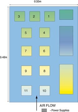
figure 3: multi-component, non-uniform array test
board schematic (air flow above & below board).
figure 4 is a comparison of computed and measured component temperatures as a function of approach velocity for a series of tests in which all 11 components were powered at 2 watts. these results were obtained after the modeling parameters (e.g. convection conductances) were tuned to best meet the experimental measurements taken at 1.25 m/sec approach velocity. this illustration shows that once a model is calibrated using one or a few data points, it can be used to provide thermal characterization data over a wide parameter space.

figure 4: comparison of measured and predicted components temperatures
as a function of air approach velocity (t-ambient=room ambient).
closure
these simple, engineering models still have a place in electronic thermal management. admittedly, their initial development will take some time. however, once in hand, they can be used to estimate performance as a function of system-level design variation variations. they are useful for interpreting and reducing the number of characterization measurements. finally, since they are based on straightforward, albeit approximate, physics-based models, they are useful for checking the sanity of more complex cfd calculations.
vincent p. manno
department of mechanical engineering
tufts university, 204 anderson hall, medford, ma 02155
tel: +1 (617) 627-5000 x 2548
fax: +1 (617) 627-3058
email: [email protected]
references
| 1. |
a. bar-cohen and w.b. krueger, "thermal characterization of chip packages - evolutionary development of compact models", thirteenth annual semiconductor thermal measurement and management symposium - semitherm xiii, austin, tx, january 28-30, 1997 ieee, pp. 180-197. |
| 2. |
c.j.m. lasance, "thermal resistance: an oxymoron?", electronics cooling, vol. 3, no.2, may 1997, pp. 20-22. |
| 3. |
h.i. rosten et al., "final report to semitherm xiii on the european-funded project delphi - the development of libraries and physical models for an integrated design environment", thirteenth annual semiconductor thermal measurement and management symposium - semitherm xiii austin, tx, january 28-30, 1997, ieee, pp. 73-91. |
| 4. |
f. kreith and m.s. bohn, principles of heat transfer, fifth edition (revised printing), pws publishing, 1997, pp. 593-594. |
| 5. |
b.m. guenin, r.c. marrs and r.j. molnar, "analysis of a thermally enhanced ball grid array package", ieee transactions on components, manufacturing, and packaging technology - part a, vol. 18, no. 4, 1995, pp. 749-757. |
|