|
introduction
uncertainty analysis is the process of estimating the uncertainty in a result calculated from measurements with known uncertainties. uncertainty analysis uses the equations by which the result was calculated to estimate the effects of measurement uncertainties on the value of the result.
uncertainty analysis is used in the planning stages of an experiment to judge the suitability of the instrumentation; during the data-taking phase to judge whether the scatter on repeated trials is "normal" or means that something has changed; and in reporting the results, to describe the range believed to contain the true value.
the mathematics of uncertainty analysis is based on the statistical treatment of error but using uncertainty analysis does not require knowledge of statistics. the possible errors in each measurement are assumed "normally distributed"; the error in each measurement is assumed independent of the error in any other measurement, and the error in every measurement is described at the same confidence level. the procedures described herein are for "single-sample" uncertainty analysis: uncertainty estimates are calculated for each data set, individually. when many data sets are averaged before the result is calculated, different equations are used.
the mathematical background
the standard form for expressing a measurement is:
 (1) (1)
this is interpreted as follows: the odds are 20/1 that the true value of x is within +/-  x of the recorded value. assuming the true value is fixed by the process, and therefore remains constant, eq. 1 means that if a large number measurements (each with a different measurement error) were made at the same test condition, using a wide variety of instruments (each with a different calibration error), the results would most likely center around the recorded value and have a "normal" distribution with a standard deviation of x of the recorded value. assuming the true value is fixed by the process, and therefore remains constant, eq. 1 means that if a large number measurements (each with a different measurement error) were made at the same test condition, using a wide variety of instruments (each with a different calibration error), the results would most likely center around the recorded value and have a "normal" distribution with a standard deviation of  x/2. x/2.
when the result is a function of only one variable, the uncertainty in the result is:
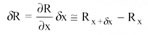 (2) (2)
the numerical approximation to the uncertainty in r is found by calculating the value of r twice: once with x augmented by  x and once with the value of x at its recorded value, and subtracting the values. x and once with the value of x at its recorded value, and subtracting the values.
when more than one measurement is used in calculating the result, r, the uncertainty in r can be estimated in two ways: "worst case combination" and "constant odds".
the "worst case combination" is highly unlikely (400/1 against, tbr two variables each at 20/1 ), what is generally wanted is the uncertainty in the result, at the same odds used in estimating the measurement errors: the "constant odds" combination. this can be achieved by:
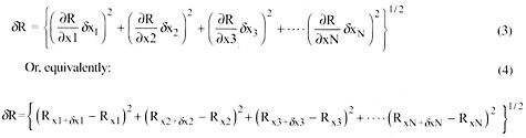
in executing eq. 4, each term is calculated with only one variable augmented by its uncertainty interval, all others being at their recorded values. eq. 3 is the classical analytical form for uncertainty analysis. it requires a separate set of equations for calculating the uncertainty. as an experiment evolves with experience, it is hard to ensure that the uncertainty equation set is kept current. when eq. 4 is used, the uncertainty analysis is always current. furthermore, the uncertainty is always calculated for every data set. on-line uncertainty analysis keeps the uncertainty in the results constantly visible, making it less likely that highly uncertain results will escape unnoticed.
table 1
calculating the uncertainty in h by sequentially perturbing the inputs to a spreadsheet sequentially perturbed data
|
input
|
est. unc.
|
data
|
|
in each col., the title variable has been increased by its uncertainty
|
|
variables
|
|
|
w
|
a
|
to
|
tcool
|
tboard
|
twall
|
stef-boltz
|
emmis
|
k
|
|
w
|
0.5
|
4.000
|
4.500
|
4.000
|
4.000
|
4.000
|
4.000
|
4.000
|
4.000
|
4.000
|
4.000
|
|
(indicated) watts
|
|
a,m2
|
2.50e-06
|
0.002
|
0.002
|
0.002
|
0.002
|
0.002
|
0.002
|
0.002
|
0.002
|
0.002
|
0.002
|
|
to, c
|
1
|
80.000
|
80.000
|
80.000
|
81.000
|
80.000
|
80.000
|
80.000
|
80.000
|
80.000
|
80.000
|
|
tcool, c
|
2
|
40.000
|
40.000
|
40.000
|
40.000
|
42.000
|
40.000
|
40.000
|
40.000
|
40.000
|
40.000
|
|
tboard, c
|
2
|
55.000
|
55.000
|
55.000
|
55.000
|
55.000
|
57.000
|
55.000
|
55.000
|
55.000
|
55.000
|
|
twall, c
|
2
|
55,000
|
55.000
|
55.000
|
55.000
|
55.000
|
55.000
|
57.000
|
55.000
|
55.000
|
55.000
|
|
stef/bolt z
|
0
|
0.000
|
0.000
|
0.000
|
0.000
|
0.000
|
0.000
|
0.000
|
0.000
|
0.000
|
0.000
|
|
emissivit y
|
0.1
|
0.800
|
0.800
|
0.800
|
0.800
|
0.800
|
0.800
|
0.800
|
0.800
|
0.900
|
0.800
|
|
sh fact, k
|
0.01
|
0.060
|
0.060
|
0.060
|
0.060
|
0.060
|
0.060
|
0.060
|
0.060
|
0.060
|
0.070
|
|
q-cond
|
|
1.500
|
1.500
|
1.500
|
1.560
|
1.500
|
1.380
|
1.500
|
1.500
|
1.500
|
1.750
|
|
q-rad
|
|
0.287
|
0.287
|
0.287
|
0.300
|
0.287
|
0.287
|
0.266
|
0.287
|
0.323
|
0.287
|
|
wact
|
|
3.920
|
4.410
|
3.920
|
3.920
|
3.920
|
3.920
|
3.920
|
3.920
|
3.920
|
3.920
|
|
qconv
|
|
2.133
|
2.623
|
2.133
|
2.060
|
2.133
|
2.253
|
2.154
|
2.133
|
2.097
|
1.883
|
|
h(i)
|
|
33.330
|
40.987
|
33.272
|
31.407
|
35.085
|
35.205
|
33.654
|
33.330
|
32.770
|
29.424
|
|
indiv cont
|
|
|
7.656
|
-0.059
|
-1.923
|
1.754
|
1.875
|
0.323
|
0.000
|
- 0.560
|
-3.906
|
|
squared
|
|
|
58.618
|
0.003
|
3.698
|
3.077
|
3.516
|
0.104
|
0.000
|
0.314
|
15.259
|
|
abs uncert
|
|
9.197
|
|
|
|
|
|
|
|
|
|
|
rel uncert
|
|
28%
|
|
|
|
|
|
|
|
|
|
calculating the uncertainty
to illustrate the process, consider an experiment measuring the average heat transfer coefficient to an electrically heated model of a component on a circuit board. the surrogate component is assumed to radiate to its surroundings, and conduct to the board. the electrical power to the component is measured using a wattmeter that requires correction. the local temperatures of the component, the coolant, the board, and the walls of the enclosure are measured using thermo-couples. conduction heal loss is estimated using a conduction shape factor and the difference between the component and the board temperature.
the radiation heat loss is calculated using the "tiny body" approximation, using the surface emissivity of the component. conduction and radiation losses are subtracted from the corrected wattmeter reading to determine the convective heat transfer rate, and h is calculated based on the difference between component temperature and coolant temperature.
the names of the data items are listed in column 1. the uncertainties associated with those measurements are in col. 2 and the measured values in col. 3. the next 9 columns are "pseudo" data sets; each made by perturbing one of the observed data bits by its uncertainty interval. the perturbed values are set in bold-faced type.
the first 5 lines in the second block calculate the conduction and radiation heat losses, the electrical power to the component, the convective heat transfer rate, and the apparent value of h. the value of h listed in col. 3 is the "nominal'' value: h calculated using the observed data. block copying lhese equations across the 9 columns of perturbed data generates 9 additional estimates of h, one for each perturbed variable. the contribution to the overall uncertainty made by each variable is found by subtracting the nominal h from the perturbed h for that variable. the root-sum-square of the individual contributions is the uncertainty in h (col. 3, abs. uncert.). the relative uncertainty is the absolute uncertainty divided by the nominal value.
interpreting the calculated uncertainty
this same spreadsheet could be used to estimate several different kinds of uncertainty depending on what kind of uncertainty estimates were provided in col. 2. the uncertainty calculated in col. 3 is always the same type as the inputs used in col. 2: fixed errors, random errors, or uncertainties. if they were uncertainties, they could have been zeroth order, first order, or nth order. the meaning of the calculated uncertainty cannot be interpreted until the type of input has been established.
fixed error: an error is considered "fixed" if its value is always the same on repeated observations at the same test condition with the same instruments and the same procedure. fixed errors must often be estimated based on what is known about the precision of the instrument's calibration, hence are often not statistically justifiable. the value used for the residual fixed error, after calibration, must have the same meaning as the 2 value (the 95% confidence level or 20/1 odds value) which would have been expected had the calibrations been repeated many times. value (the 95% confidence level or 20/1 odds value) which would have been expected had the calibrations been repeated many times.
random error: an error is considered "random" if its value is different on subsequent observations, and the difference varies randomly from trial to trial. there are few truly random processes above the molecular level. what appears to be random variation usually represents merely slow sampling of a fast process. in any case, the value used to describe the "random" error is the 2σ value expected for the population of measurements which might have been made.
uncertainty: the uncertainty in a measurement is defined as the root-sum-square of its fixed error and its random error, as described above. it represents the interval within which the true value is believed to lie, accounting for both fixed and random errors.
zeroth order uncertainty: the uncertainty represented by the fixed and random errors introduced by the instrumentation alone, with no contribution from the process. the zeroth order uncertainty is used to judge the fitness of the proposed instruments for the intended experiment. if the uncertainty in the result is unacceptably large, calculated using zeroth order inputs, then better instruments must be obtained.
first order uncertainty: the uncertainty contributed by short-term instability of the process as viewed through the instrumentation. first order uncertainty includes both process instability and the random component of instrument error. it is assessed by taking a set of 30 or more observations over a representative interval of time with the system running normally, using the normal instrumentation, and calculating the standard deviation of the set, σ. the first order uncertainty is 2σ. first order uncertainty estimates are used to judge the significance of scatter on repeated trials. if more than one of 20 repeated trials falls outside the first order interval, this may suggest system changes.
nth order uncertainty: the overall uncertainty in the measurement accounting for process instability and the fixed and random errors in the instrumentation. nth order uncertainty is calculated as the root-sum-square of the fixed errors due to the instrumentation and the first order uncertainty. it represents the total range, around the reported value, within which the true value is believed to lie. the nth order uncertainty is used in reporting the results in the literature, or comparing the presented result with a result from some other facility, or with some absolute truth (such as a conservation of energy test). the n thorder uncertainty should not be used to assess the significance of scatter, since the fixed errors do not change on repeated trials.
interpreting the spreadsheet
in the present example, the nominal value of h is 33.3 w/m2oc with an uncertainty of 9.2 w/m2oc .
- if each input provided in col. 2 represents the estimated fixed errors in that measurement, then the 9.2 represents the fixed error in h.
- if each input provided in col. 2 represents the 2σ value from a set of repeated readings during the instrument's calibration, then the 9.2 represents the instrumentation's contribution to the random error in h.
- if each input provided in col. 2 is the root-sum-square of the fixed and random error in the instrumentation, then the 9.2 represents the zeroth order uncertainty - the instrumentation's contribution to the overall uncertainty in h.
- if each input provided in col. 2 is the 2σ value from a set of observations made with the system running, then the 9.2 represents the first order uncertainty in the result - the scatter which should be expected on repeated trials if the system does not change.
- if each input provided in col. 2 is the root-sum-square of the fixed error due to the instrumentation and the first order uncertainty, then the 9.2 represents the nth order uncertainty in the result - the interval within which the true value is believed to lie.
robert j. moffat
stanford university
menlo park, ca
selected readings
1. moffat, r.j., "contributions to the theory of single-sample uncertainty analysis," trans. asme, journal of fluids engineering, vol. 104, no. 2, pp. 250-260, june 1982.
2 . taylor, james l., fundamentals of measurement error, neff instrument corporation, 1988.
3. dieck, ronald h. measurement, uncertainty - methods and applications, instrument society of america, 1992.
4. ansl/asme ptc 19.1-1985, instruments and apparatus, part 1, measurement uncertainty.
references:
1 . azar, k., and russell, e.t., effect of component layout and geometry on flow distribution in electronic circuit packs. asme journal of electronic packaging, vol. 113, p. 50-57, march 1991.
2 . wijk, j.j. van, a.j.s. hin, w.c. de leeuw, f.h. post, three ways to show 3d fluid flow. ieee computer graphics and applications, vol. 14, no. 5, p. 33~39, september 1994.
3 . cabral, b. and l. leedom, imaging vector fields using line integral convolution. proceedings siggraph'93, computer graphics, vol.27, no.4, p.263-270, 1993.
4. wijk, j.j. van, spot noise - texture synthesis for data visualization. proceedings slggraph'91, computer graphics, vol. 25, no.4, p.309-318, 1991.
5 . leeuw, w.c. de, and r. van liere, divide and conquer spot noise. proceedings super computing '97, san jose, november 1997, acm slgarch.
6. wijk, j.j. van, flow visualization with surface particles. ieee computer graphics and applications, vol. 13, no. 4, p. 18-24, july 1993.
7. banks, d.c. and b.a. singer, vortex tubes in turbulent flows: identification, representation, reconstruction. proceedings of ieee visualization '94, p. 132-139, cs press, 1994.
8. helman, j.l. and l. hesselink, visualizing vector field topology in fluid flows. ieee computer graphics and applications , vol. 11, no. 3, p. 36-46, may 1991.
|